Confidentiality in microdata.no

Background

The Act on Official Statistics and Statistics Norway (LOV-2019-06-21-32) § 14 (access to information for statistical results and analyzes) section (5) states that "The duty of confidentiality pursuant to § 8 applies correspondingly to the person who has access to information". Such data can only be provided to researchers in approved research institutions or to public authorities. Therefore, strict requirements are imposed on the supply of data for research and an application for access to microdata for research is a long process. You can find the criteria for applying for access to research data for research at Statistics Norway's pages on data for research.

The microdata.no analysis system is designed to make it possible to access microdata from registers without having to go through the lengthy application process for obtaining data. But it is a condition for such a simplification that the security and confidentiality of the microdata are as well taken care of as when delivered, preferably better. It has therefore been an explicit requirement from the outset that users should not be able to view microdata or otherwise be able to disclose information about individuals. When Statistics Norway publishes official statistics, this is aggregated data. Nevertheless, Statistics Norway must make sure through various types of measures that it is not possible to disclose information about individuals or other types of statistical units to which the statistics relate.

The results/output that microdata.no produces for its users (tables or analyzes) are, like Statistics Norway's statistics, aggregated data. But without limitations, a user of microdata.no could easily produce tables and other types of statistical results that Statistics Norway would not be able to publish. To prevent this from happening, several types of measures have been introduced that will limit the possibilities of being able to disclose information that should be confidential.

This appendix will describe the measures implemented to safeguard confidentiality in microdata.no. The measures are based on scenarios on how the confidentiality of microdata.no can be attacked or accidentally compromised. These scenarios will not be described. Emphasis will however be placed on what is necessary, in order for the user to understand the measures implemented and properly relate to the statistical results.

The measures described below are those that have been implemented so far. There will be more measures added over time or even adjustments to the measures described below. This appendix will be updated when changes occur.

Measure 1: Minimum population size

It is not allowed to define populations with fewer than 1000 people. Attempts to define such will be met with an error message of the type

Measure 2: Winsorization

Winsorization is a technique often used in analyses to prevent extreme observations from having too much influence on the analysis results. The technique is applied to all numerical variables and consists of cutting the distribution at both ends by specific percentiles. We use 2% winsorization which means that the 1% highest values ​​are set to the 99-percentile (lower limit value) and the 1% lowest values ​​are set to the 1-percentile (upper limit value). This only happens when displaying statistical results, based on the current population from which the statistics are calculated.

The distributions for many numerical statistical variables will be skewed, typically with long tails at the upper end (e.g. income or wealth). Therefore, winsorization will affect average and standard deviations to a certain degree. Both types of statistics will typically be estimated too low. On the other hand, medians, quartiles and other percentiles will not be affected.

Example: Consider the following script where the goal is to create descriptive statistics and histograms for the age distribution of the population as of 2010.

 import BEFOLKNING_FOEDSELS_AAR_MND as faarmnd
generate faar = floor(faarmnd/100)
drop faarmnd
generate alder2010 = 2010 - faar
summarize alder2010
histogram alder2010, discrete
 

Note: faarmnd = birth year and month (*YYYYMM*), and alder2010 = age per 2010

The result will look like this:

summarize alder2010

Variabel	mean	std	count	1%	25%	50%	75%	99%
alder2010	38.7467	22.681	255743	1	21	37	55	89

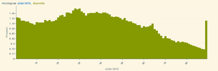
Anyone older than 89 years will be set to 89, and 0 year olds will be set to 1 year. This is the cause of the large bar to the right of the histogram. We are aware that the winsorization can create problems when studying the elders. The same applies to studies of other groups that are defined by belonging to the tail in the distribution for a numerical variable.

Winsorization affects all statistics and graphical plots, and prevents the most extreme values ​​from being visible.

Results produced through regression analyses are not to be considered as personally identifiable information. Such analyses therefore use the underlying non-winsorized data. Regression estimates will therefore not be affected by winsorization.

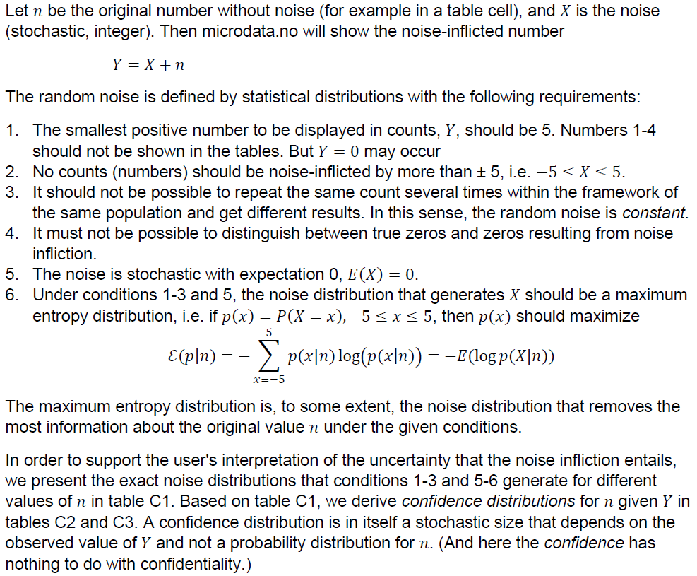
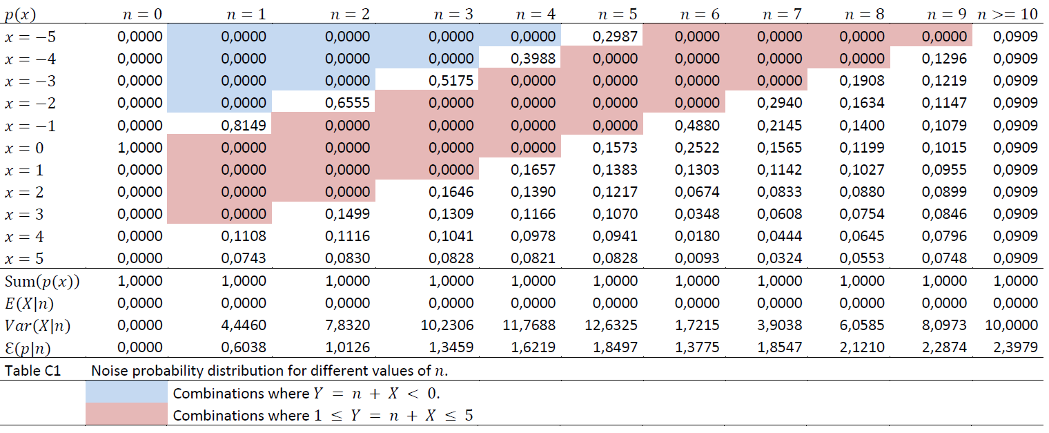
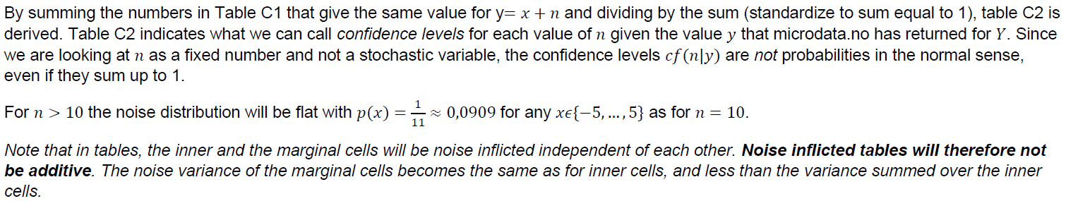
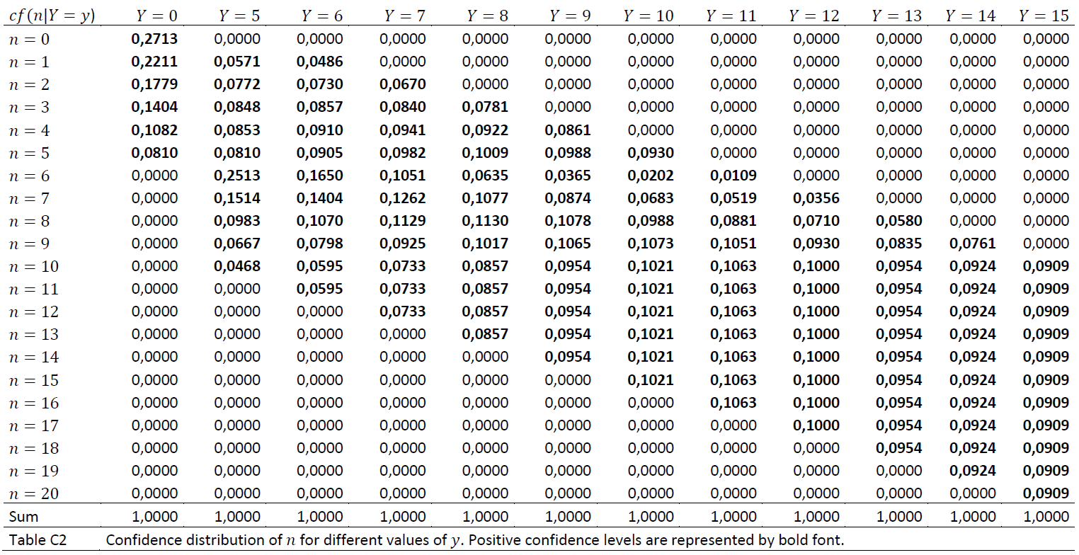
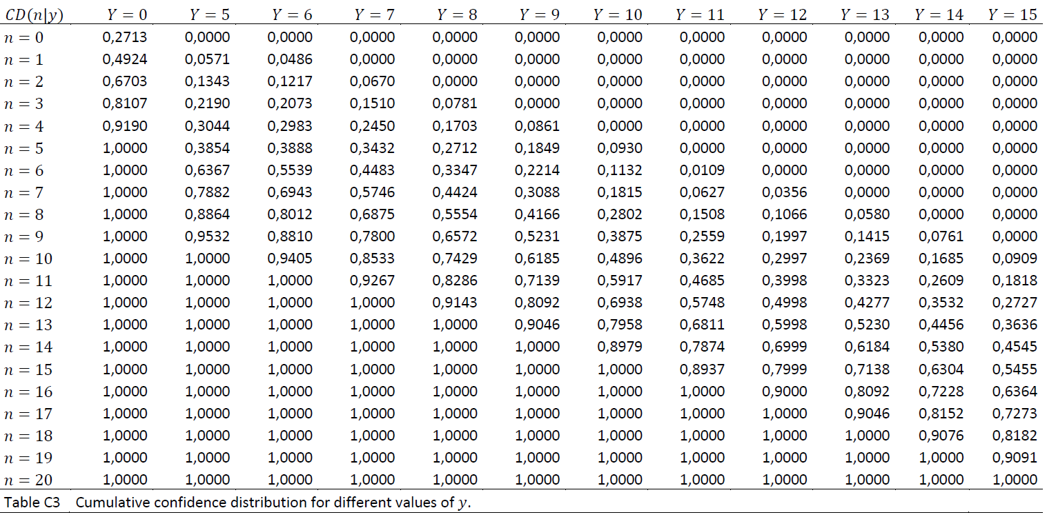
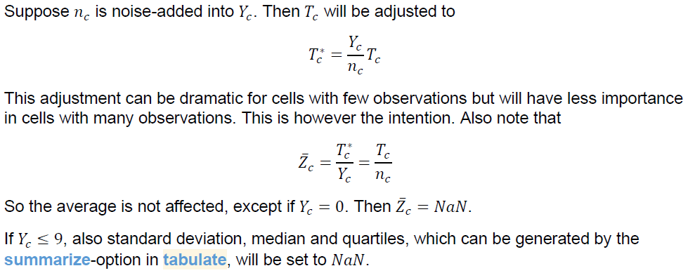
Measure 3: Randomized noise

All counts of the number of units in a dataset that are shown related to various operations, or statistical counts presented through commands such as tabulate or summarize are noise-inflicted. Summations of numerical statistics variables associated with the units in a table cell, such as income, will be adjusted proportionally to the noise factor so that average numbers are unaffected. Where the random noise results in the number of units behind the sum being 0, the sum is set to 0 and the average, which then becomes 0/0 is set to NaN.

Measure 4: Graphic plots - Hexbin plots

It is common to use scatter plot diagrams to establish a visual image of data or to show the relationship between numerical variables. Such plots can be very revealing, especially if there are few observations in relation to the graphical area or in areas outside the main mass of points. If, for a given unit/person in the population, the value of one of the variables that span out the plot is known, it will often be possible to read the value of the second variable with too much accuracy.

To prevent this from happening, we have in microdata.no chosen to smooth such plots with a smoothing technique. For this purpose, we have attempted to focus on a technique called hexbin plot. In a hexbin plot, the graphic area is divided into regular hexagons.

Example of hexbin plot made in microdata.no:

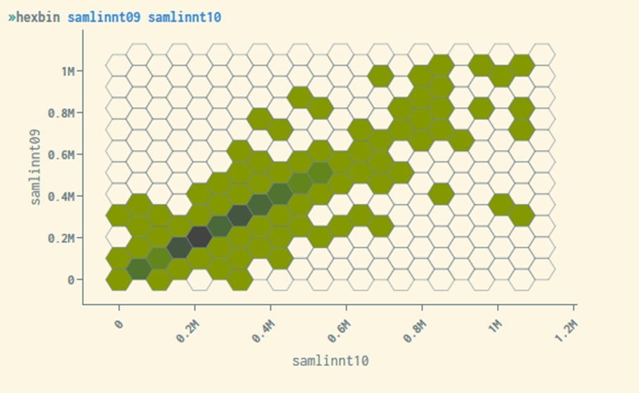Figure C1. Hexbin plot showing total income in 2009 vs. 2010 for a small population

In a hexbin plot, the graphical area is scaled based on the largest and smallest values ​​that occur for the variables being plotted. The largest and smallest values ​​are influenced by the winsorization referred to in measure 2. The hexagons are given a colour or hue indicating an interval for how many units there are in them, for example 30-59, 60-89, etc. The range of units/ persons each hue represents are equally long and are automatically adjusted according to the distribution in the data.

Hexbin plot is under trial. In the current version, all hexagons where the number of people is less than 20% of the most populated hexagon form are blanked. This criterion will be adjusted as soon as it is possible to give priority. Note that the winsorization of the numerical variables that span the plot will affect the plot.

Measure 5: Hiding tables with too many low values

Tables created by the tabulate command may in some cases contain many cells with low values ​​for the number of units. This can be problematic as it makes it easier to indirectly identify individuals by studying combinations of values ​​for the categorical variables that make up a table. Another problem with such tables is that the noise generation described under «Measure 3» gives a relatively high uncertainty for the relevant cell values ​​(the percentage noise becomes relatively large with small numbers), so that the statistical usefulness of the table is low.

In microdata.no, a limit value of 50% is operated, i.e. tables where more than 50% of the cells contain frequency values ​​lower than 5 will be stopped. In addition, an error message about this will be displayed.

It is possible to avoid the problem of tables being stopped due to many low cell values: By making coarser divisions for the categorical variables that make up the table, or by increasing the size of the table population, you will be able to increase the number of units in each cell and thus fall below the 50% limit so that the table is approved and displayed.

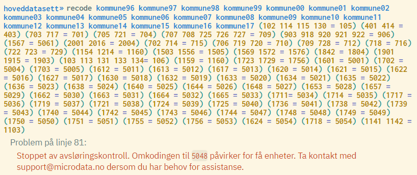
Measure 6: No changes affecting fewer than 10 units are allowed

It is not allowed to make changes to a data set that affect fewer than 10 units, through the use of the commands generate, replace or recode(). If this occurs, you will receive an error message and the execution will stop.

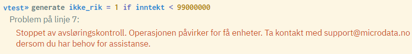
It is also not allowed to make changes that affect all units except a number less than 10.

Examples:

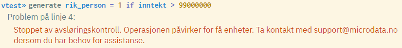
("rik_person" = "rich person", "ikke_rik" = "not rich", "inntekt" = "income", "Stoppet av avsløringskontroll. Operasjonen påvirker for få enheter." = "Stopped due to disclosure control. This operation affects too few units.")

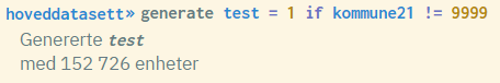
An important exception is that you can make changes that affect all or no units.

Examples (the code 9999 for municipality is not existing in the dataset):

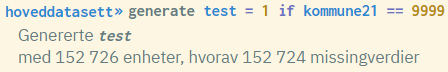
(Note that the number of missing values ​​reported is different from the number of units in the example above. This is due to the noise of frequency values, cf. Measure 3. In practice, the variable test will only contain missing values.)

By using recode, then the rule applies to each of the recoding terms in the expression (each of the recode rules/terms are checked, i.e. the to-code, and each of them must recode at least 10 observations).

Example:

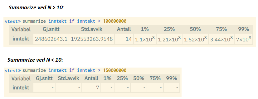
Measure 7: Descriptive statistics are not permitted for populations of fewer than 10

Descriptive statistics through the commands summarize or summarize in combination with tabulate cannot be run on populations of fewer than 10. Exceptions are sums and frequencies.

Example:

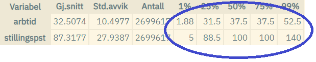
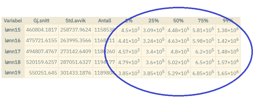
Measure 8: Median and percentile values ​​are displayed with three-digit precision only

Median and percentile values ​​show actual values ​​that can be linked to individuals (or other entities). Therefore, such values ​​are only displayed with three-digit precision, and affect the display of numbers when using the commands summarize, summarize in combination with tabulate, and graphs where such numbers are included.

Examples:

Measure 9: Constant terms are hidden from regression results if the analysis population has too unique combinations of categorical values

In order to strengthen the confidentiality of regression analyses, we have introduced a restriction relating to analyses on datasets with too high a degree of uniqueness. If combinations of categorical variable values ​​in the analysis form very small groups, the constant term estimates will be hidden from the regression results. The analysis is not affected since the constant term is included in the estimation.

It is the principle of k-anonymity that is used on the underlying analysis dataset, defined by the population and the set of explanatory variables for the analysis in question, where the limit value is set to 5. Concealment of constant terms thus occurs for regressions that are run on datasets with fewer than 5 units with same combination of variable values.

Note that continuous variables are not included in assessments of uniqueness, only categorical variables.

In cases where measure 9 comes into play, and you want to see the constant term, there are some steps you can take to make the dataset less unique (so that the number of unique combinations exceeds 5):

• Increase the population size
• Use a coarser division of categories
• Limit the number of categorical explanatory variables