5.2 ANOVA
ANOVA analyses can be seen as a simplified linear regression analysis, where you examine whether the mean value of a continuous variable is different in two or more groups given by a categorical grouping variable. One possible example is testing whether the mean wage is different for people with low, medium and high education (using a variable where education level is divided into three groups).
Syntax:
anova <variable> <variable list> [if <condition>] [, <options>]
Example:

The example above shows a simple analysis with only one grouping variable, i.e. a one-way ANOVA analysis. This shows that there is a significant difference in yearly wage ("lønn") between the categories of gender ("kjønn"), i.e. between men and women. This is seen from the p-value of the F-test being equal to 0 (i.e. below 0.05). You can also test the continuous variable against two other categorical variables. This is called a two-way ANOVA analysis.
By using the posthoc option, you can run a post hoc analysis and in addition make pairwise comparisons of the average of the categorical variable measured across all the respective categories for the grouping variable. This means that each individual category is compared directly with all the other categories:
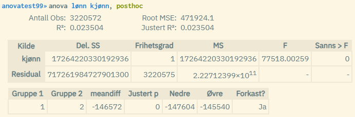
The post hoc analysis also shows what the difference in the average wage is between the two categories of male and female given by the values 1 and 2. In addition, an adjusted p-value is shown that shows whether the difference is significant (p-value below 0.05). If it says "Ja" (Yes) in the column "Forkast?" (Reject?), this means that the null hypothesis of no difference is rejected. A confidence interval is also shown for each comparison.
Post hoc can also be used on two-way ANOVA analysis (then the list of pairwise comparisons is expanded to include the additional variable):
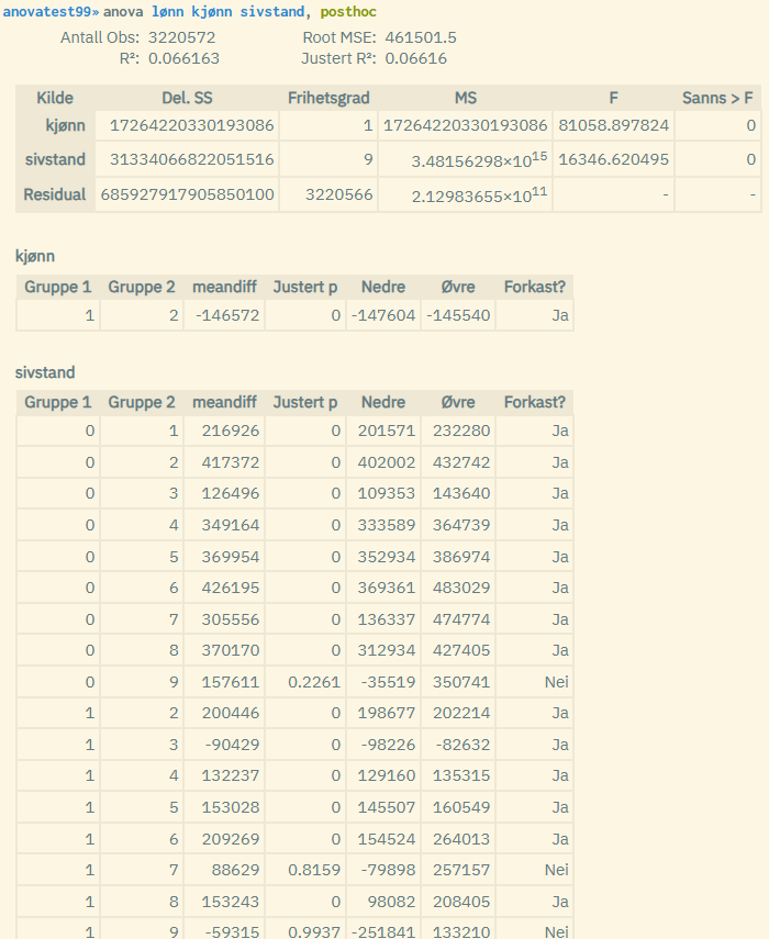
In the extended two-way ANOVA with post hoc, both the variables gender and marital status are checked. The marital status variable has 10 categories, and the list of pairwise comparisons becomes much longer (the entire table does not fit in this example view). As you can see, there are significant differences between most marital status categories, but not all. For example, there is no significant difference between marital status categories 0 and 9, 1 and 7, or 1 and 9.
In chapter 5.4, you can read more about linear regression analyses. These take it a step further and estimate the effect of each category on a continuous variable (response variable) in relation to a base/reference category for a given categorical variable (explanatory variable), where you control for a set of other variables that also have an effect. In other words, you say something about whether there is a positive, negative, or no effect (in relation to a reference category), instead of just comparing means. Linear regression analyses can also be used to look at the effect on a continuous variable (response variable) of a unit increase in one or more continuous variables (explanatory variables).
Source:
The algorithms for the anova command are based on the function anova_lm, which takes the result of an OLS estimation on the same variables as the input. The posthoc option uses a TukeyHSD approximation based on the function pairwise_tukeyhsd. Both functions are found in the Statsmodels module in Python.